Allometry with R and ggplot2
This web page was created based on using the blogdown and Hugo packages to publish an R Markdown document. Markdown is a simple formatting syntax for authoring HTML, PDF, and MS Word documents. For more details on using R Markdown see http://rmarkdown.rstudio.com.
In the text below, you should be able to copy all of the code in the gray code chunks and paste it into a script file to replicate the results and figures in R on your own computer.
Making a figure demonstrating the metabolic allometry of social insect colonies
#	loading libraries
library(ggplot2)
library(scales)

#	Importing the raw data
#	Doing this with dput() on a data set I previously assembled instead of making you import a separate data file.  For simplicity, so you can execute this whole page of code without needing anything else.

scaling.data <- structure(list(Mass_g = c(1.4, 1.7002, 1.8, 1.9434, 2.1375, 2.1416,
2.499, 2.5802, 2.82, 3.14, 3.15, 3.2887, 3.9303, 3.9844, 4.5304,
6.22, 11.15, 0.5831, 2.1449, 2.3775, 2.4805, 2.772, 2.83, 3.2861,
3.6833, 4.12, 4.2299, 4.4661, 7.23, 8.05, 11.12, 14.07, 15.994,
16.52, 23, 35, 0.026297706, 0.040436744, 0.044237498, 0.045942821,
0.062768431, 0.07691959, 0.065188108, 0.065188108, 0.066432704,
0.095607687, 0.102634562, 0.109658189, 0.104100736, 0.104100736,
0.102150441, 0.119965244, 0.149818237, 0.183594797, 0.169415356,
0.297376027, 0.187100058, 0.211573861, 0.316227766, 0.524460187,
0.615924842, 0.502611051, 0.502611051, 0.455104241, 0.455104241,
2.2228, 1.0851, 0.311, 1.0518, 1.947, 1.339, 1.7183, 1.8048,
1.8124, 0.3163, 0.4948, 1.0259, 0.4044, 0.199643, 0.129236, 0.171042,
0.073814, 0.216383228, 0.428173, 0.0735, 0.02291, 0.306489, 0.02648,
0.035914, 0.215908, 0.5765, 0.37279, 0.28873, 0.11961, 0.055239,
4.55, 9, 9.5, 20, 28, 46.5, 55.8, 56.7, 85.1, 93.3, 164, 170,
179, 195, 416, 438, 603, 839, 1150), MetRate_uW = c(11725, 10887.5,
11334.1666666667, 12221.9166666667, 14684.1666666667, 10775.8333333333,
17531.6666666667, 13902.5, 17587.5, 14963.3333333333, 17140.8333333333,
18648.3333333333, 23896.6666666667, 24120, 25236.6666666667,
28084.1666666667, 35621.6666666667, 6700, 13232.5, 14740, 19876.6666666667,
21719.1666666667, 26409.1666666667, 24734.1666666667, 27805,
23561.6666666667, 27079.1666666667, 30875.8333333333, 28810,
31545.8333333333, 45895, 66218.3333333333, 53516.25, 57675.8333333333,
71020, 79283.3333333333, 33.7753585, 30.92522114, 27.53816388,
26.65809962, 32.69596607, 39.00034792, 42.59470698, 45.24307437,
62.31533437, 53.71694463, 53.71694463, 53.71694463, 60.88626912,
67.11765019, 90.74424905, 85.82973089, 87.43759511, 77.14186669,
100.9640395, 92.01623324, 149.0857861, 146.3442914, 166.6475603,
178.6593132, 201.5666172, 207.2570381, 238.2114803, 255.3814733,
360.0043728, 2416.22338, 1440.06502, 381.9876907, 1162.588857,
2473.06643, 1777.550277, 2571.259972, 1251.548476, 1988.6147,
684.5054588, 847.744214, 1094.032191, 720.4679038, 1275.378835,
862.7678496, 1036.910662, 664.1199683, 1148.200077, 5802.41761,
426.9794844, 411.6824213, 2421.204683, 556.5702842, 501.2094544,
2049.271617, 4622.855531, 3281.145231, 2225.307599, 959.549531,
524.668946, 214411.1667, 368835, 341057.9167, 740350, 1009913.333,
1090425, 1000075.5, 949725, 1192605.583, 1479427, 1263620, 1898333.333,
1828932.5, 2743650, 2369120, 3105785, 3501420, 3513312.5, 5168770.833
), Species = structure(c(2L, 2L, 2L, 2L, 2L, 2L, 2L, 2L, 2L,
2L, 2L, 2L, 2L, 2L, 2L, 2L, 2L, 1L, 1L, 1L, 1L, 1L, 1L, 1L, 1L,
1L, 1L, 1L, 1L, 1L, 1L, 1L, 1L, 1L, 1L, 1L, 13L, 13L, 13L, 13L,
13L, 13L, 13L, 13L, 13L, 13L, 13L, 13L, 13L, 13L, 13L, 13L, 13L,
13L, 13L, 13L, 13L, 13L, 13L, 13L, 13L, 13L, 13L, 13L, 13L, 12L,
12L, 12L, 12L, 12L, 12L, 12L, 12L, 12L, 12L, 12L, 12L, 12L, 11L,
11L, 11L, 11L, 11L, 11L, 11L, 11L, 11L, 11L, 11L, 11L, 11L, 11L,
11L, 11L, 11L, 14L, 14L, 14L, 14L, 14L, 14L, 14L, 14L, 14L, 14L,
14L, 14L, 14L, 14L, 14L, 14L, 14L, 14L, 14L), .Label = c("Camponotus rufipes",
"Odontomachus bauri", "Za", "Anoplolepis steinergroeveri", "Atta columbica",
"Camponotus fulvopilosus", "Camponotus maculatus", "Eciton hamatum",
"Formica rufa", "Messor pergandei", "Pheidole dentata", "Pogonomyrmex californicus",
"Temnothorax rugatulus", "Apis mellifera"), class = "factor"),
    Unit = structure(c(1L, 1L, 1L, 1L, 1L, 1L, 1L, 1L, 1L, 1L,
    1L, 1L, 1L, 1L, 1L, 1L, 1L, 1L, 1L, 1L, 1L, 1L, 1L, 1L, 1L,
    1L, 1L, 1L, 1L, 1L, 1L, 1L, 1L, 1L, 1L, 1L, 1L, 1L, 1L, 1L,
    1L, 1L, 1L, 1L, 1L, 1L, 1L, 1L, 1L, 1L, 1L, 1L, 1L, 1L, 1L,
    1L, 1L, 1L, 1L, 1L, 1L, 1L, 1L, 1L, 1L, 1L, 1L, 1L, 1L, 1L,
    1L, 1L, 1L, 1L, 1L, 1L, 1L, 1L, 1L, 1L, 1L, 1L, 1L, 1L, 1L,
    1L, 1L, 1L, 1L, 1L, 1L, 1L, 1L, 1L, 1L, 1L, 1L, 1L, 1L, 1L,
    1L, 1L, 1L, 1L, 1L, 1L, 1L, 1L, 1L, 1L, 1L, 1L, 1L, 1L), .Label = c("Colony",
    "Worker ant"), class = "factor"), Type = structure(c(2L,
    2L, 2L, 2L, 2L, 2L, 2L, 2L, 2L, 2L, 2L, 2L, 2L, 2L, 2L, 2L,
    2L, 1L, 1L, 1L, 1L, 1L, 1L, 1L, 1L, 1L, 1L, 1L, 1L, 1L, 1L,
    1L, 1L, 1L, 1L, 1L, 6L, 6L, 6L, 6L, 6L, 6L, 6L, 6L, 6L, 6L,
    6L, 6L, 6L, 6L, 6L, 6L, 6L, 6L, 6L, 6L, 6L, 6L, 6L, 6L, 6L,
    6L, 6L, 6L, 6L, 5L, 5L, 5L, 5L, 5L, 5L, 5L, 5L, 5L, 5L, 5L,
    5L, 5L, 4L, 4L, 4L, 4L, 4L, 4L, 4L, 4L, 4L, 4L, 4L, 4L, 4L,
    4L, 4L, 4L, 4L, 8L, 8L, 8L, 8L, 8L, 8L, 8L, 8L, 8L, 8L, 8L,
    8L, 8L, 8L, 8L, 8L, 8L, 8L, 8L), .Label = c("Camponotus rufipes",
    "Odontomachus bauri", "Za", "Pheidole dentata", "Pogonomyrmex californicus",
    "Temnothorax rugatulus", "Worker ant", "Apis mellifera"), class = "factor")), .Names = c("Mass_g",
"MetRate_uW", "Species", "Unit", "Type"), row.names = c(1L, 2L,
3L, 4L, 5L, 6L, 7L, 8L, 9L, 10L, 11L, 12L, 13L, 14L, 15L, 16L,
17L, 18L, 19L, 20L, 21L, 22L, 23L, 24L, 25L, 26L, 27L, 28L, 29L,
30L, 31L, 32L, 33L, 34L, 35L, 36L, 37L, 38L, 39L, 40L, 41L, 42L,
43L, 44L, 45L, 46L, 47L, 48L, 49L, 50L, 51L, 52L, 53L, 54L, 55L,
56L, 57L, 58L, 59L, 60L, 61L, 62L, 63L, 64L, 65L, 66L, 67L, 68L,
69L, 70L, 71L, 72L, 73L, 74L, 75L, 76L, 77L, 78L, 79L, 80L, 81L,
82L, 83L, 84L, 85L, 86L, 87L, 88L, 89L, 90L, 91L, 92L, 93L, 94L,
95L, 226L, 227L, 228L, 229L, 230L, 231L, 232L, 233L, 234L, 235L,
236L, 237L, 238L, 239L, 240L, 241L, 242L, 243L, 244L), class = "data.frame")

#	Inspect data frame
head(scaling.data)
##   Mass_g MetRate_uW            Species   Unit               Type
## 1 1.4000   11725.00 Odontomachus bauri Colony Odontomachus bauri
## 2 1.7002   10887.50 Odontomachus bauri Colony Odontomachus bauri
## 3 1.8000   11334.17 Odontomachus bauri Colony Odontomachus bauri
## 4 1.9434   12221.92 Odontomachus bauri Colony Odontomachus bauri
## 5 2.1375   14684.17 Odontomachus bauri Colony Odontomachus bauri
## 6 2.1416   10775.83 Odontomachus bauri Colony Odontomachus bauri
str(scaling.data)
## 'data.frame':	114 obs. of  5 variables:
##  $ Mass_g    : num  1.4 1.7 1.8 1.94 2.14 ...
##  $ MetRate_uW: num  11725 10888 11334 12222 14684 ...
##  $ Species   : Factor w/ 14 levels "Camponotus rufipes",..: 2 2 2 2 2 2 2 2 2 2 ...
##  $ Unit      : Factor w/ 2 levels "Colony","Worker ant": 1 1 1 1 1 1 1 1 1 1 ...
##  $ Type      : Factor w/ 8 levels "Camponotus rufipes",..: 2 2 2 2 2 2 2 2 2 2 ...

#	Plotting the raw data
ggplot(scaling.data, aes(x=Mass_g, y=MetRate_uW)) + geom_point()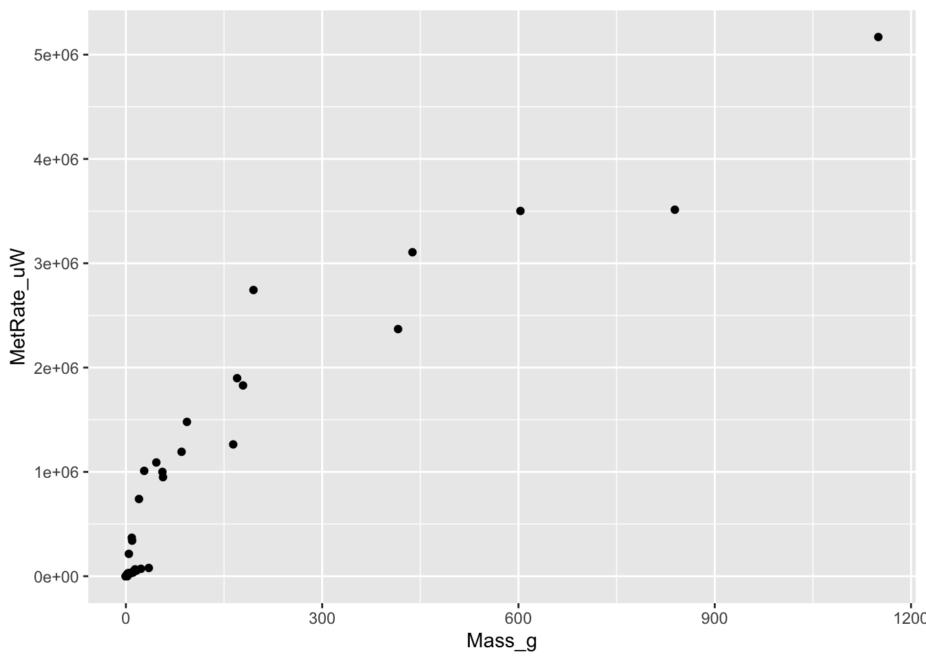
#	Log-transforming the data on x- and y-axes
ggplot(scaling.data, aes(x=log10(Mass_g), y=log10(MetRate_uW))) + geom_point()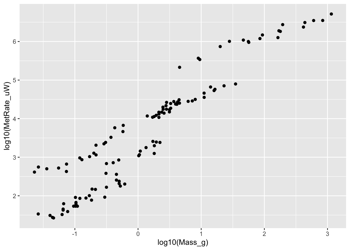
#	Adding color codes and regression lines
ggplot(scaling.data, aes(x=log10(Mass_g), y=log10(MetRate_uW), color=Type)) + geom_point() + stat_smooth(method="lm")
## `geom_smooth()` using formula = 'y ~ x'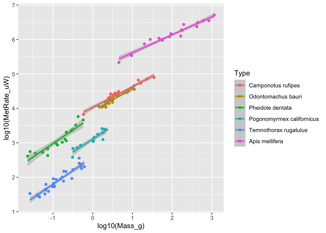
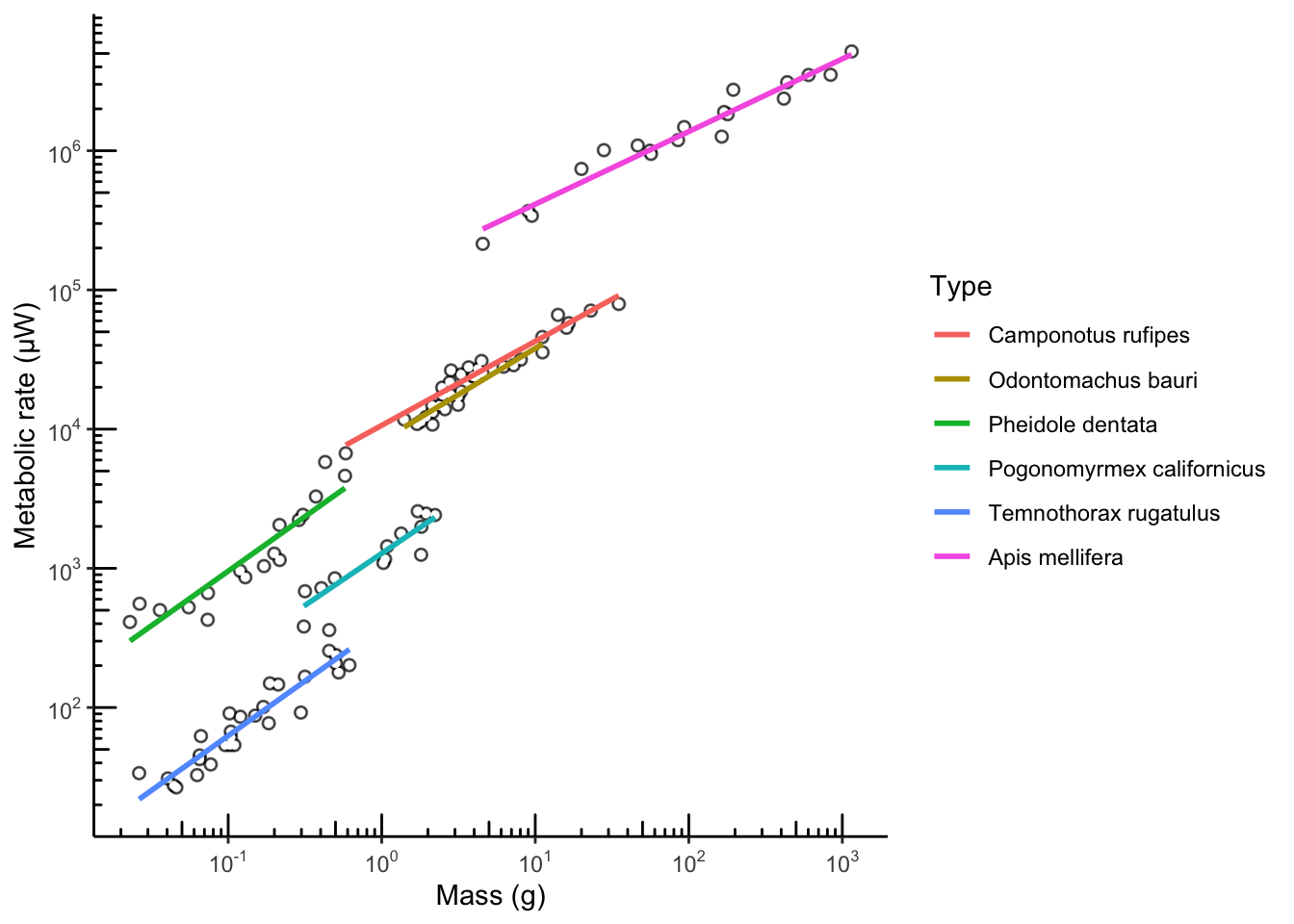
#	Making it fancy by adding
#	 - log ticks on the axes
#	 - axes labels appropriate for log transformed data
#	 - simplifying the ggplot theme look

ggplot(scaling.data, aes(x=log10(Mass_g), y=log10(MetRate_uW), color=Type))  + geom_point(size=1, color="grey80") + annotate("point", x=log10(scaling.data$Mass_g[scaling.data$Unit == "Colony"]), y=log10(scaling.data$MetRate_uW[scaling.data$Unit == "Colony"]), color="black", size=2, alpha=0.6) + annotate("point", x=log10(scaling.data$Mass_g[scaling.data$Unit == "Colony"]), y=log10(scaling.data$MetRate_uW[scaling.data$Unit == "Colony"]), color="white", size=1) + geom_smooth(method="lm", se=F) + theme_bw() + theme(panel.grid.minor = element_blank()) + scale_x_continuous(name = "Mass (g)", labels = math_format(10^.x)) + scale_y_continuous(name = "Metabolic rate (µW)", labels = math_format(10^.x)) + annotation_logticks(sides="lb") + theme(panel.grid.major=element_blank(), panel.border=element_blank())+ theme(axis.line = element_line())
## `geom_smooth()` using formula = 'y ~ x'